Local Mean Surface Temperature#
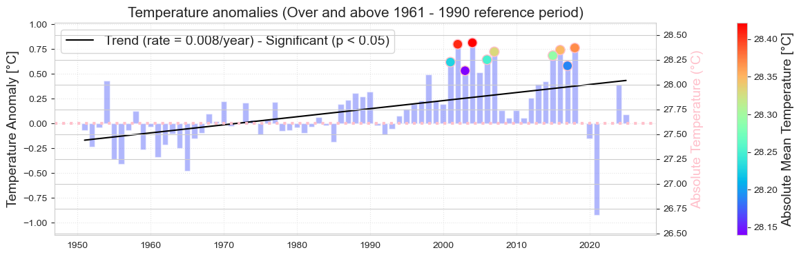
Figure: Annual mean temperature anomalies relative to 1961–1990 climatology at Koror. The colored dots represent the 10 warmest years on record, with the absolute values shown along the right axis. The solid black line represents the trend, which is statistically significant (p < 0.05). From NOAA ESRL Global Monitoring Division. https://www.esrl.noaa.gov/gmd/ccgg/trends/
Setup#
First, we need to import all the necessary libraries. Some of them are specifically developed to handle the download and plotting of the data and are hosted at the indicators set-up repository in GitHub
Show code cell source
import warnings
warnings.filterwarnings("ignore")
Show code cell source
import os.path as op
import sys
import contextlib

import numpy as np
import pandas as pd
import matplotlib.pyplot as plt

from myst_nb import glue

sys.path.append("../../../../indicators_setup")
from ind_setup.plotting_int import plot_timeseries_interactive, fig_int_to_glue
from ind_setup.plotting import plot_bar_probs, fontsize

sys.path.append("../../../functions")
from data_downloaders import GHCN, download_oni_index, filter_by_time_completeness

from ind_setup.plotting_int import plot_oni_index_th
from ind_setup.plotting import plot_bar_probs_ONI, add_oni_cat
Define location and variables of interest#
country = 'Palau'
vars_interest = ['TMIN', 'TMAX']
Get Data#
update_data = False
path_data = "../../../data"
path_figs = "../../../matrix_cc/figures"
Observations from Koror Station#
https://www.ncei.noaa.gov/data/global-historical-climatology-network-daily/doc/GHCND_documentation.pdf
The data used for this analysis comes from the GHCN (Global Historical Climatology Network)-Daily database.
This a database that addresses the critical need for historical daily temperature, precipitation, and snow records over global land areas. GHCN-Daily is a
composite of climate records from numerous sources that were merged and then subjected to a suite of
quality assurance reviews. The archive includes over 40 meteorological elements including temperature daily maximum/minimum, temperature at observation time,
precipitation and more.
The next code blocks download the data and postprocess it to generate an easy to use dataframe with all the variables of interest for the analysis.
Show code cell source
if update_data:
    df_country = GHCN.get_country_code(country)
    print(f'The GHCN code for {country} is {df_country["Code"].values[0]}')

    df_stations = GHCN.download_stations_info()
    df_country_stations = df_stations[df_stations['ID'].str.startswith(df_country.Code.values[0])]
    print(f'There are {df_country_stations.shape[0]} stations in {country}')
Show code cell source
if update_data:
    GHCND_dir = 'https://www.ncei.noaa.gov/data/global-historical-climatology-network-daily/access/'
    id = 'PSW00040309' # Koror Station
    dict_min = GHCN.extract_dict_data_var(GHCND_dir, 'TMIN', df_country_stations.loc[df_country_stations['ID'] == id])[0][0]
    dict_max = GHCN.extract_dict_data_var(GHCND_dir, 'TMAX', df_country_stations.loc[df_country_stations['ID'] == id])[0][0]
    st_data = pd.concat([dict_min['data'], (dict_max['data'])], axis=1).dropna()
    st_data['diff'] = st_data['TMAX'] - st_data['TMIN']
    st_data['TMEAN'] = (st_data['TMAX'] + st_data['TMIN'])/2
    st_data.to_pickle(op.join(path_data, 'GHCN_surface_temperature.pkl'))
else:
    st_data = pd.read_pickle(op.join(path_data, 'GHCN_surface_temperature.pkl'))
# Inclusion criteria: remove months/years with less than 75% of data

df_filt, removed_months, removed_years = filter_by_time_completeness(
    st_data,
    month_threshold=0.75,
    year_threshold=0.75
)
print(f"Removed {removed_months.shape[0]} months due to insufficient data: {removed_months.index.tolist()}")
print(f"Removed {removed_years.shape[0]} years due to insufficient data: {removed_years.index.tolist()}")

st_data = df_filt #replace data with filtered data
st_data_daily = st_data.copy()
Removed 14 months due to insufficient data: [(2018, 8), (2019, 1), (2020, 3), (2022, 7), (2022, 10), (2022, 11), (2022, 12), (2023, 1), (2023, 6), (2023, 8), (2023, 12), (2024, 2), (2025, 8), (2025, 10)]
Removed 3 years due to insufficient data: [2019, 2022, 2023]
st_data = st_data.resample('YE').mean()
glue("n_years", len(np.unique(st_data.index.year)), display=False)
glue("start_year", st_data.dropna().index[0].year, display=False)
glue("end_year", st_data.dropna().index[-1].year, display=False)
Analysis#
Plotting#
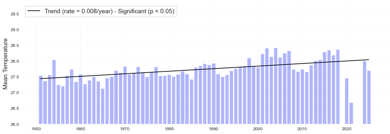
At this piece of code we will plot the Mean annual temperature over time and its associated trend
dict_plot = [{'data' : st_data, 'var' : 'TMEAN', 'ax' : 1, 'label' : 'TMEAN'},
        ]
dict_plot = [{'data' : st_data, 'var' : 'TMEAN', 'ax' : 1, 'label' : 'TMEAN'}]
fig = plot_timeseries_interactive(dict_plot, trendline=True, figsize = (25, 12))

glue("trend_fig_mean", fig_int_to_glue(fig), display=False)
Fig. Annual maxima corresponding to the mean temperature.
fig, ax, trend = plot_bar_probs(x = st_data.index.year, y = st_data['TMEAN'].values , trendline = True,
               figsize = (15, 5), y_label = f'Mean Temperature', return_trend = True)
ax.set_ylim(26, None)
(26.0, 29.842663934426227)
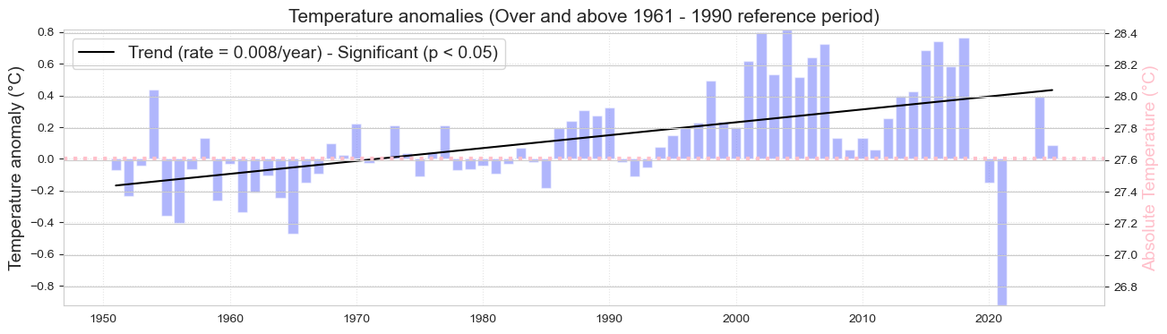
Here we are creating a new column with the information of the temperature refered to the climatology of 1960 to 1990
mean_ref = st_data.loc['1961':'1990'].TMEAN.mean()
st_data['TMEAN_ref'] = st_data['TMEAN'] - mean_ref
import matplotlib.pyplot as plt
fig, ax, trend = plot_bar_probs(x = st_data.index.year, y = st_data.TMEAN_ref, trendline = True, figsize = [15, 4], return_trend = True)
ax.set_ylim(st_data.TMEAN_ref.min(), st_data.TMEAN_ref.max())
ax2 = ax.twinx()
ax2.axhline(mean_ref, color='pink', linestyle=':', linewidth=3)
ax2.set_ylim(st_data.TMEAN_ref.min() + mean_ref, st_data.TMEAN_ref.max()+ mean_ref)
ax2.set_ylabel('Absolute Temperature (°C)', fontsize = fontsize, color = 'pink')
ax.set_ylabel('Temperature anomaly (°C)', fontsize = fontsize)
plt.title('Temperature anomalies (Over and above 1961 - 1990 reference period)', fontsize = 15);
nevents = 10
top_10 = st_data.sort_values(by='TMEAN_ref', ascending=False).head(nevents)
The following bar plot represents the mean temperature anomalies with respect to the 1960-1990 climatology along with the 10 largest temperature events in the record
fig, ax, trend = plot_bar_probs(x=st_data.index.year, y=st_data.TMEAN_ref, trendline=True,
                                y_label='Temperature Anomaly [°C]', figsize=[15, 4], return_trend=True)


ax.set_ylim(st_data.TMEAN_ref.min()-.2, st_data.TMEAN_ref.max()+.2)
ax2 = ax.twinx()
ax2.axhline(mean_ref, color='pink', linestyle=':', linewidth=3)
ax2.set_ylim(st_data.TMEAN_ref.min()-.2 + mean_ref, st_data.TMEAN_ref.max() + .2 + mean_ref)
ax2.set_ylabel('Absolute Temperature (°C)', fontsize = fontsize, color = 'pink')

glue("trend_mean", float(trend), display=False)
glue("change_mean", float(trend * len(np.unique(st_data.index.year))), display=False)
glue("top_10_year", float(top_10.sort_index().index.year[0]), display=False)

im = ax2.scatter(top_10.index.year, top_10.TMEAN,
                c=top_10.TMEAN.values, s=100, ec = 'pink', cmap='rainbow', label='Top 10 warmest years')
plt.title('Temperature anomalies (Over and above 1961 - 1990 reference period)', fontsize=15)
plt.colorbar(im, pad = .1).set_label('Absolute Mean Temperature [°C]', fontsize=fontsize)
plt.savefig(op.join(path_figs, 'F2_ST_Annomalies_top10.png'), dpi=300, bbox_inches='tight')
glue("trend_fig", fig, display=False)
Fig. 1 Annomaly of the mean temperature over and above the 1961-1990 reference period. Overlapping points correspond to the top 10 warmer years.#
El Niño Southern Oscillation Analysis#
ONI index#
The Oceanic Niño Index (ONI) is the standard measure used to monitor El Niño and La Niña events. It is based on sea surface temperature anomalies in the central equatorial Pacific (Niño 3.4 region) averaged over 3-month periods.
https://origin.cpc.ncep.noaa.gov/products/analysis_monitoring/ensostuff/ONI_v5.php
p_data = 'https://psl.noaa.gov/data/correlation/oni.data'
df1 = download_oni_index(p_data)
lims = [-.5, .5]
plot_oni_index_th(df1, lims = lims)
st_data_monthly = st_data_daily.resample('M').mean()
st_data_monthly.index = pd.DatetimeIndex(st_data_monthly.index).to_period('M').to_timestamp() #+ pd.offsets.MonthBegin(1)
df1['tmin'] = st_data_monthly['TMIN']
df1['tmax'] = st_data_monthly['TMAX']
df1['tdiff'] = df1['tmax'] - df1['tmin']
df1['tmean'] = (df1['tmax'] + df1['tmin'])/2
df1['tmean_ref'] = df1['tmean'] - df1.loc['1961':'1990'].tmean.mean()
df1['tmean_ref_min'] = df1['tmean'] - df1.groupby(df1.index.year).max().tmean.min()
df1 = add_oni_cat(df1, lims = lims)
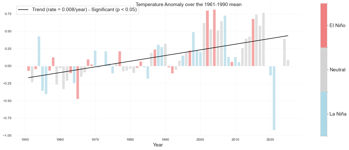
The following bar plot represents the mean temperature anomalies with respect to the 1960-1990 climatology. The color of the bar represents wether it is a El Niño or La Niña year.
df2 = df1.resample('Y').mean()
fig = plot_bar_probs_ONI(df2, var='tmean_ref');
fig.suptitle('Temperature Anomaly over the 1961-1990 mean', fontsize = fontsize)
plt.savefig(op.join(path_figs, 'F2_ST_Mean.png'), dpi=300, bbox_inches='tight')
# glue("fig_ninho", fig, display=False)
df_format = np.round(df1.describe(), 2)
Generate table#
Table sumarizing different metrics of the data analyzed in the plots above
from ind_setup.tables import style_matrix, table_temp_11
style_matrix(table_temp_11(df2, trend))
| Metric | Value |
|---|---|
| Mean Temperature | 27.728 |
| Change in Annual Mean Temperature since 1951 | 0.600 |
| Rate of Change (°C/year) | 0.008 |