Degree Heating Weeks

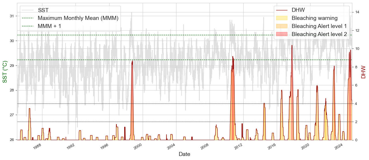
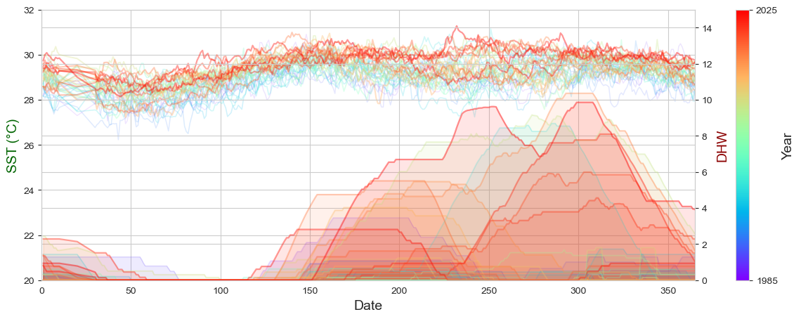
Figure. NOAA Coral Reef Watch Degree Heating Weeks at the virtual station in the vicinity of Palau. The Degree Heating Week (DHW) value is shown on the vertical axis on the right. The coral bleaching heat stress level (or Bleaching Alert Level) – Warning, Alert Level 1, Alert Level 2 – are color-coded and shaded-in along the bottom horizontal axis. Red dashed lines across the graphs indicate DHW threshold values of 4- and 8-degree Celsius-weeks (triggers for Bleaching Alert Levels 1 and 2, respectively). The representative SST value is shown on the vertical axis on the left. The monthly mean climatology, the MMM, and the bleaching threshold SST are also provided on the graph.

Show code cell source Hide code cell source

import warnings
warnings.filterwarnings("ignore")

import sys
import os
import os.path as op

import geopandas as gpd
import pandas as pd
import matplotlib.pyplot as plt
from myst_nb import glue

sys.path.append("../../../../indicators_setup")
from ind_setup.plotting import plot_dhw, plot_dhw_perpetual_year, plot_dhw_bleaching_levels, add_oni_cat

sys.path.append("../../../functions")
from ocean import process_bleaching_levels
from data_downloaders import download_oni_index

Setup

Define area of interest

path_data = "sst_daily_1981_2024_palau.nc"
path_figs = "../../../matrix_cc/figures"

lon_site, lat_site = 134.368203, 7.322074

# Area of interest
lon_range = [129.4088, 137.0541]
lat_range = [1.5214, 11.6587]

EEZ shapefile

shp_f = op.join(
    os.getcwd(), "..", "..", "..", "data/Palau_EEZ/pw_eez_pol_april2022.shp"
)
shp_eez = gpd.read_file(shp_f)

Download Data

The NOAA Coral Reef Watch (CRW) daily global 5km satellite coral bleaching Degree Heating Week (DHW) product for the virtual station in the vicinity of Palau shows accumulated heat stress, which can lead to coral bleaching and death (Figure 15). Bleaching heat stress is categorized into risk levels based on the DHW values, which are directly related to the timing and intensity of coral bleaching – Bleaching Warning (0 < DHW < 4), Bleaching Alert Level 1 (4 <= DHW < 8), and (8 <= DHW < 12). At Bleaching Alert Level 1, significant bleaching is expected within a few weeks of the alert. At Bleaching Alert Level 2 and above, severe, widespread bleaching and significant coral mortality are likely.

https://coralreefwatch.noaa.gov/product/5km/methodology.php#dhw

Show code cell source Hide code cell source

"""
Name:
Palau
Polygon Middle Longitude:
134.4250 
Polygon Middle Latitude:
7.6750  
Averaged Maximum Monthly Mean:
29.2309
Averaged Monthly Mean (Jan-Dec):
28.0424 27.7264 27.8581 28.4679 29.1780 29.2309 28.8550 28.7810 28.8377 29.0823 29.1088 28.8078
First Valid DHW Date:
1985 25 03
First Valid BAA Date:
1985 31 03
"""
data_crw = pd.read_csv(
    "https://coralreefwatch.noaa.gov/product/vs/data/palau.txt", sep=r"\s+", skiprows=20
)
data_crw.to_csv("data_crw_palau.csv")
data_crw.index = pd.to_datetime(
    data_crw["YYYY"].astype(str)
    + data_crw["MM"].astype(str)
    + data_crw["DD"].astype(str),
    format="%Y%m%d",
)
data_crw = data_crw.groupby(level=0).max()
# data_crw = data_crw[~data_crw.index.duplicated()]
data_crw.sort_index(inplace=True)
# data_crw = data_crw.resample('W').mean()
data_crw = data_crw[:"2024"]

Analysis

Stress Level

No Stress HotSpot <= 0
Bleaching Watch 0 < HotSpot < 1
Bleaching Warning 1 <= HotSpot and 0 < DHW < 4
Bleaching Alert Level 1 1 <= HotSpot and 4 <= DHW < 8
Bleaching Alert Level 2 1 <= HotSpot and 8 <= DHW

Full time period

fig, ax2 = plot_dhw(data_crw)
plt.savefig(op.join(path_figs, "F13_DHW.png"), dpi=300, bbox_inches="tight")
glue("dhw_all", fig, display=False)

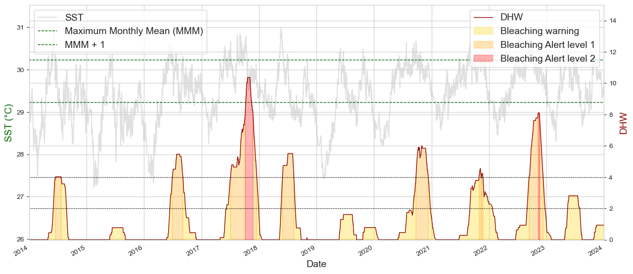
Last 10 years

fig, ax2 = plot_dhw(data_crw)
ax2.set_xlim("2014", "2024")

(np.float64(16071.0), np.float64(19723.0))

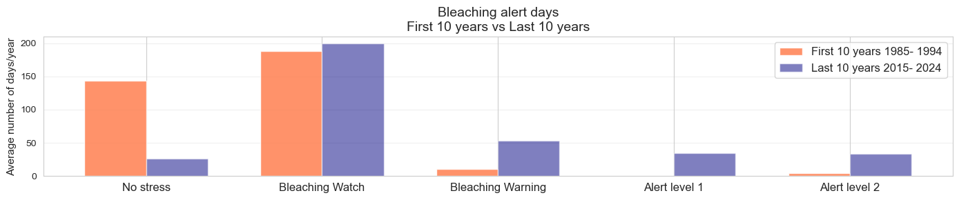
Bleaching alert levels: change

df, days_pivot = process_bleaching_levels(data_crw)

days_pivot/10

period	First 10 years	Last 10 years
bleaching_level
No stress	143.8	26.0
Bleaching Watch	187.9	199.8
Bleaching Warning	11.1	53.0
Alert level 1	0.0	34.9
Alert level 2	4.4	33.6

fig = plot_dhw_bleaching_levels(df, days_pivot)

df

	YYYY	MM	DD	SST_MIN	SST_MAX	SST@90th_HS	SSTA@90th_HS	90th_HS>0	DHW_from_90th_HS>1	BAA_7day_max	year	bleaching_level	period
1985-01-01	1985	1	1	28.12	28.32	28.26	-0.2252	0.00	0.0000	0	1985	No stress	First 10 years
1985-01-02	1985	1	2	28.03	28.29	28.24	-0.2561	0.00	0.0000	0	1985	No stress	First 10 years
1985-01-03	1985	1	3	28.18	28.42	28.36	-0.1171	0.00	0.0000	0	1985	No stress	First 10 years
1985-01-04	1985	1	4	28.27	28.50	28.43	-0.0190	0.00	0.0000	0	1985	No stress	First 10 years
1985-01-05	1985	1	5	28.16	28.40	28.37	-0.0619	0.00	0.0000	0	1985	No stress	First 10 years
...	...	...	...	...	...	...	...	...	...	...	...	...	...
2024-12-27	2024	12	27	29.67	29.95	29.84	1.3003	0.64	4.0871	1	2024	Alert level 1	Last 10 years
2024-12-28	2024	12	28	29.48	29.94	29.81	1.3745	0.55	4.0871	1	2024	Alert level 1	Last 10 years
2024-12-29	2024	12	29	29.48	29.94	29.80	1.4032	0.55	3.9429	1	2024	Bleaching Warning	Last 10 years
2024-12-30	2024	12	30	29.39	29.87	29.76	1.3426	0.48	3.9429	1	2024	Bleaching Warning	Last 10 years
2024-12-31	2024	12	31	29.52	29.84	29.74	1.1926	0.49	3.7800	1	2024	Bleaching Warning	Last 10 years

13890 rows × 13 columns

Perpetual Year

fig, ax2 = plot_dhw_perpetual_year(data_crw, yeari=1985, yeare=2025)

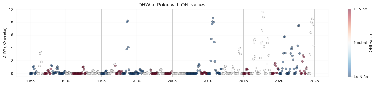
ONI index analysis

p_data = 'https://psl.noaa.gov/data/correlation/oni.data'
df1 = download_oni_index(p_data)
df1['dhw'] = df.select_dtypes(include="number").resample("MS").mean()['DHW_from_90th_HS>1']
df1 = df1.dropna()
df1 = add_oni_cat(df1, lims = [-0.5, 0.5])

df1

	ONI	dhw	oni_cat
1985-01-01	-1.04	0.000000	-1
1985-02-01	-0.85	0.000000	-1
1985-03-01	-0.77	0.000000	-1
1985-04-01	-0.78	0.000000	-1
1985-05-01	-0.78	0.120506	-1
...	...	...	...
2024-08-01	-0.07	7.948545	0
2024-09-01	-0.17	8.623337	0
2024-10-01	-0.21	8.486539	0
2024-11-01	-0.30	7.650193	0
2024-12-01	-0.42	4.291065	0

480 rows × 3 columns

fig, ax = plt.subplots(figsize=(17, 3))
# im = ax.scatter(df1.index, df1['dhw'], c=df1.ONI, s = 20, cmap = 'RdBu_r', vmin = -1, vmax = 1)
im = ax.scatter(df1.index, df1['dhw'], c=df1.oni_cat, s = 30, cmap = 'RdBu_r', ec = 'k', linewidths = .4, vmin = -1, vmax = 1, alpha = .5)
cbar = plt.colorbar(im, ax=ax, label='ONI value')
cbar.set_ticks([-1, 0, 1])
cbar.set_ticklabels(["La Niña", "Neutral", "El Niño"])
ax.set_ylabel('DHW (°C-weeks)')
ax.set_title('DHW at Palau with ONI values')

Text(0.5, 1.0, 'DHW at Palau with ONI values')