All Tropical Cyclones

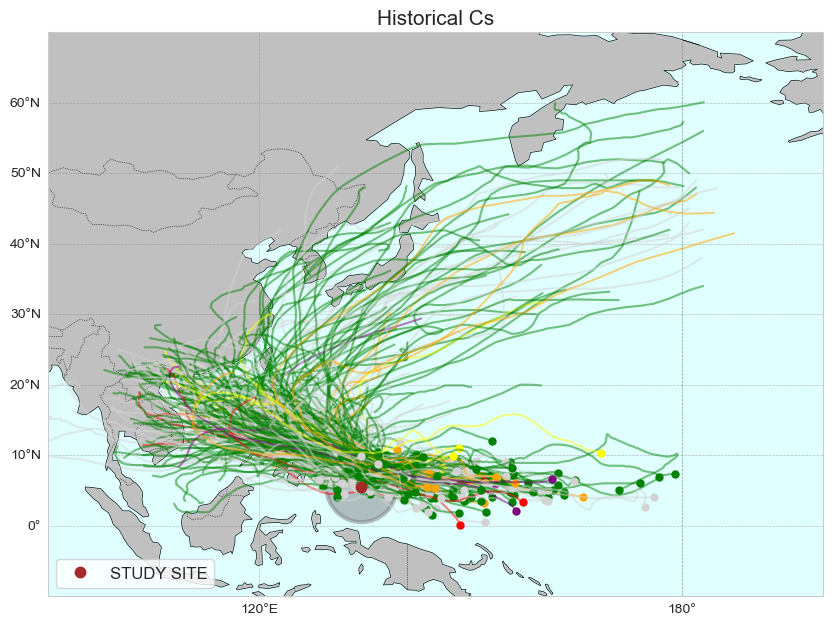
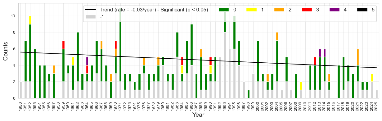
Figure. Tropical cyclones (TCs) in the vicinity of Palau since 1950. Map showing all TC tracks in the vicinity of Palau (top) and annual storm count (bottom). Categorizes are colored following the Saffir Simpson scale for wind intensity (see text for details). Grey represents TCs where no wind information is available. The dashed black line represents a trend that is not statistically significant.

In this notebook we will analyze the historical tropical cyclones in the Vicinity of Palau, as well as:

• The number of tropical cyclones per year
  

• The trend in the number of tropical cyclones over time
  

• The distribution of categories over time
  

• The influence of El Niño Southern Oscillation

Setup

First, we need to import all the necessary libraries. Some of them are specifically developed to handle the download and plotting of the data and are hosted at the indicators set-up repository in GitHub

Show code cell source Hide code cell source

import warnings
warnings.filterwarnings("ignore")
import sys
import os.path as op
import xarray as xr
import pandas as pd
from myst_nb import glue 
import numpy as np
import matplotlib.pyplot as plt

sys.path.append("../../../functions")
from tcs import Extract_Circle, get_ibtracs_category
from data_downloaders import download_ibtracs

sys.path.append("../../../../indicators_setup")
from ind_setup.plotting_tcs import Plot_TCs_HistoricalTracks_Category
from ind_setup.plotting import plot_bar_probs, plot_tc_categories_trend

from ind_setup.plotting import plot_bar_probs_ONI, add_oni_cat
from data_downloaders import  download_oni_index

lon_lat = [134.5, 5.5] #Palau location lon, lat
basin = 'WP'
r1 = 5 # Radius of the circular area in degrees

IBTrACS

IBTrACS (International Best Track Archive for Climate Stewardship) is the most comprehensive global database of tropical cyclones. It compiles data from all major meteorological agencies worldwide, providing track, intensity, and metadata for storms from 1842 to present. It supports research on cyclone trends, risks, and climate variability.

update_data = False
path_data = "../../../data"
path_figs = "../../../matrix_cc/figures"

Show code cell source Hide code cell source

if update_data:
    url = 'https://www.ncei.noaa.gov/data/international-best-track-archive-for-climate-stewardship-ibtracs/v04r01/access/netcdf/IBTrACS.ALL.v04r01.nc'
    tcs = download_ibtracs(url, basin = basin)
    tcs.to_netcdf(f"{path_data}/tcs_{basin}.nc")
else:
    tcs = xr.load_dataset(f"{path_data}/tcs_{basin}.nc")

Analysis

tcs = tcs.isel(storm = np.where(tcs.isel(date_time = 0).time.dt.year >= 1950)[0])    

Show code cell source Hide code cell source

# tcs = xr.open_dataset('/Users/laurac/Downloads/IBTrACS.ALL.v04r01.nc')

Show code cell source Hide code cell source

d_vns = {
    'longitude': 'lon',
    'latitude': 'lat',
    'time': 'time',
    'pressure': 'wmo_pres',
    'wind': 'wmo_wind',
}
tcs_sel, tcs_sel_params = Extract_Circle(tcs, lon_lat[0], lon_lat[1], r1, d_vns, fillwinds=True)

tcs_WP = get_ibtracs_category(tcs, d_vns)

/Users/laurac/Library/Mobile Documents/com~apple~CloudDocs/Projects/CC_indicators/CC_indicators/notebooks_historical/atmosphere/4_tropical_cyclones/../../../functions/tcs.py:31: RankWarning: Polyfit may be poorly conditioned
  linreg = np.polyfit(xfit[~mask], yfit[~mask], 2)

The static plot below shows all the TCs in the vicinity of Palau colored by its category.

tcs_sel_params['category'] = (('storm'), np.where(np.isnan(tcs_sel_params.category), -1, tcs_sel_params.category))
tcs_WP['category'] = (('storm'), np.where(np.isnan(tcs_WP.category), -1, tcs_WP.category))

Plotting

lon1, lon2 = 90, 200
lat1, lat2 = -10, 70

# r1
fig, ax = Plot_TCs_HistoricalTracks_Category(
    tcs_sel, tcs_sel_params.category,
    lon1, lon2, lat1, lat2,
    lon_lat[0], lon_lat[1], r1,
)

plt.savefig(op.join(path_figs, 'F8_TCs_Historical.png'), dpi=300, bbox_inches='tight')
glue("tracks_fig", fig, display=False)

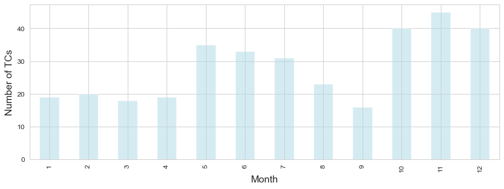
Plot of the TC count per month showing the seasonality of TC genesis in the area

import matplotlib.pyplot as plt
tcs_sel_params['month'] =  tcs_sel_params.dmin_date.dt.month
tcs_sel_params.to_dataframe().groupby('month').count().index_in.plot.bar(figsize = (12, 4), color = 'lightblue', alpha = .5)
plt.ylabel('Number of TCs', fontsize = 14)
plt.xlabel('Month', fontsize = 14)

Text(0.5, 0, 'Month')

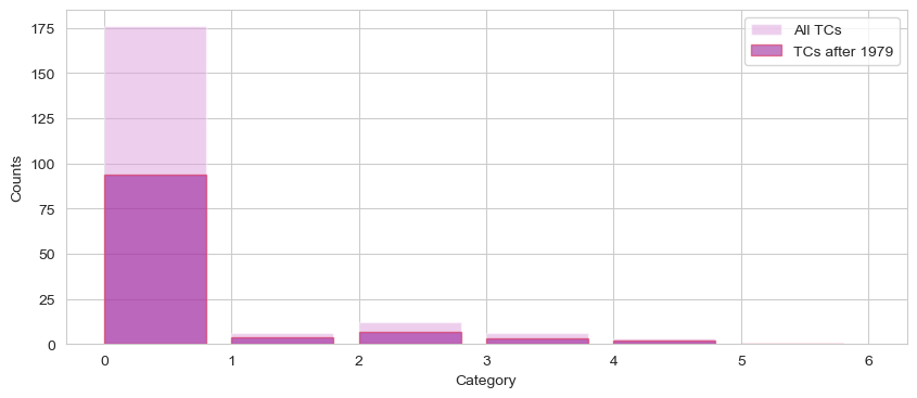
Count TCs by category

The bar plot below displays the TC count per category in the whole record and also to the record limited to 1979 and after.

u, c = np.unique(tcs_sel_params.category, return_counts=True)

import matplotlib.pyplot as plt
fig, ax = plt.subplots(1, figsize=(10, 4))
ax.grid(zorder = -1)
tcs_sel_params.category.plot.hist(bins=range(7), ax=ax, color='plum', alpha=0.5, edgecolor= None, width = .8, linewidth=1, label = 'All TCs')
tcs_sel_params.where(tcs_sel_params.dmin_date.dt.year >=1979, 
                     drop = True).category.plot.hist(bins=range(7), ax=ax, 
                                                     color='darkmagenta', alpha=0.5, edgecolor='crimson', width = .8, linewidth=1, label = 'TCs after 1979')
ax.set_xlabel('Category')
ax.set_ylabel('Counts')

ax.legend()

<matplotlib.legend.Legend at 0x18554d5e0>

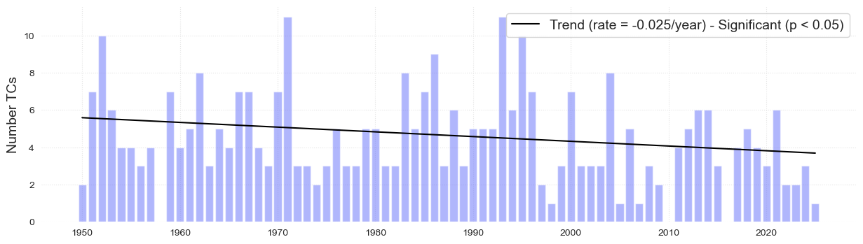
The plot below shows the trend of the number of TCs per year over time.

time = tcs_sel_params.dmin_date.dt.year.values
u, cu = np.unique(time, return_counts=True)
plot_bar_probs(x = u, y = cu, figsize= (15, 4), trendline = True,
               y_label =  'Number TCs')

(<Figure size 1500x400 with 1 Axes>, <Axes: ylabel='Number TCs'>)

The following bar plot displays the TC count per year and per category, as well as the trend.
The grey color represent those TCs in the record where no pressure or wind information is available to determine the corresponding category.

fig = plot_tc_categories_trend(tcs_sel_params, trendline_plot = False)
plt.savefig(op.join(path_figs, 'F8_TCs_Historical_bars_category.png'), dpi=300, bbox_inches='tight')
glue("time_cat_fig", fig, display=False)

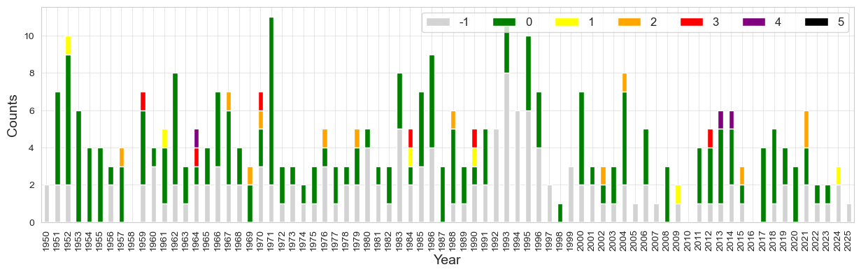
fig = plot_tc_categories_trend(tcs_sel_params, trendline_plot = True)
plt.savefig(op.join(path_figs, 'F8_TCs_Historical_bars_category.png'), dpi=300, bbox_inches='tight')
glue("time_cat_fig", fig, display=False)

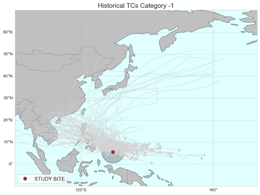
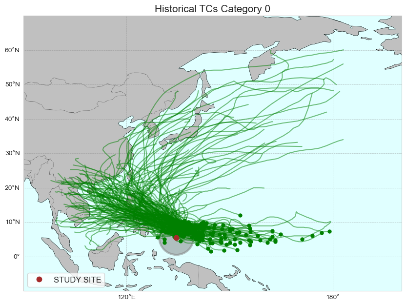
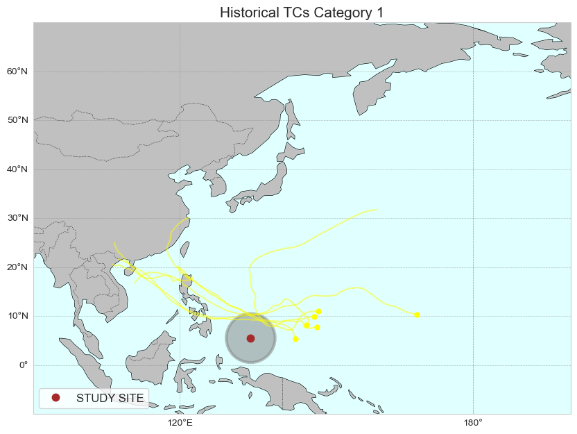
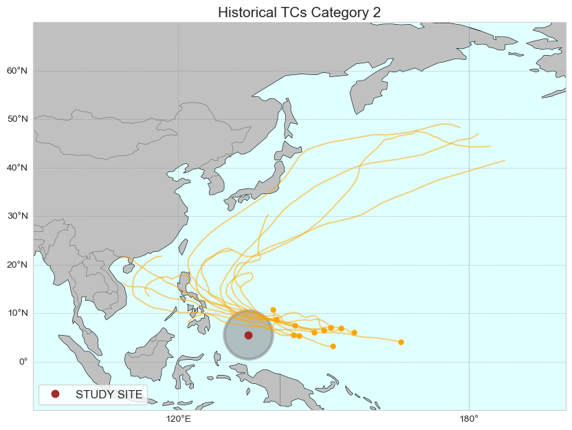
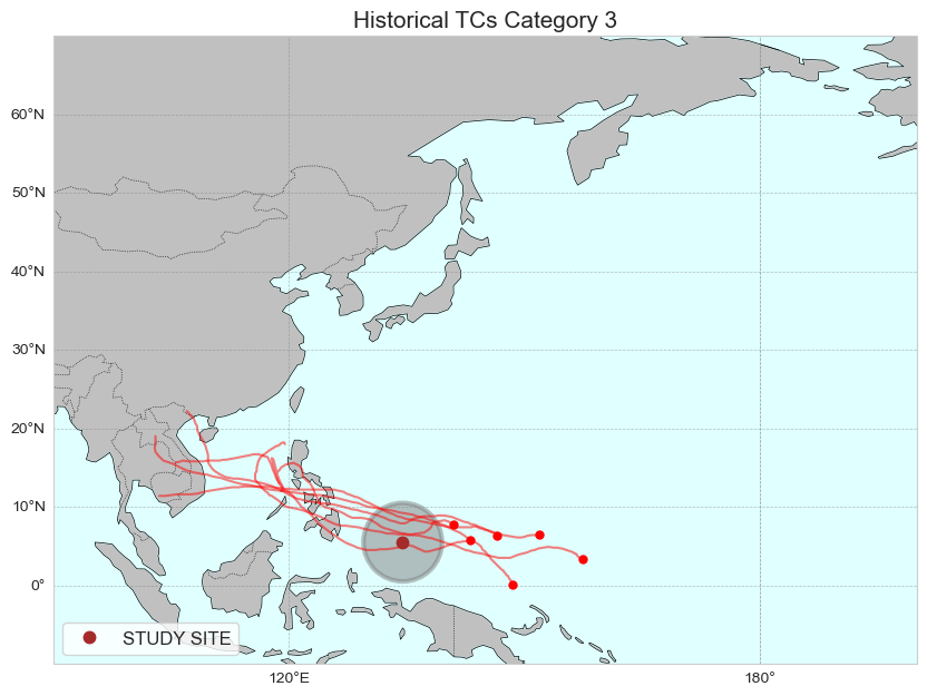
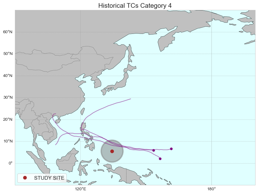
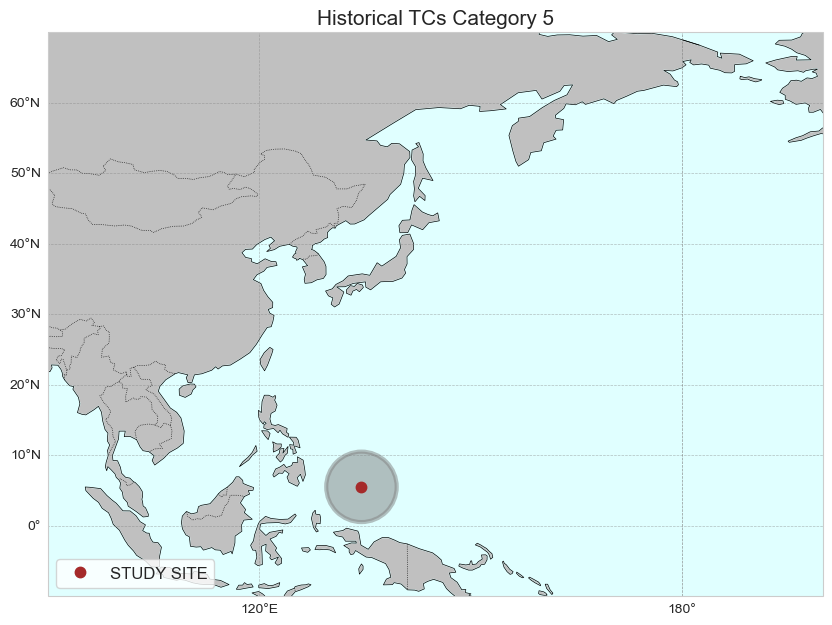
To showcase the spatial distribution of the TC tracks for the different categories, a map is shown below representing all the TCs in the record for each category.

for category in np.arange(-1, 6, 1):

    tcs_cat = tcs_sel.where(tcs_sel_params.category == category, drop = True)
    tcs_cat_params = tcs_sel_params.where(tcs_sel_params.category == category, drop = True)

    # r1
    fig, ax = Plot_TCs_HistoricalTracks_Category(
        tcs_cat, tcs_cat_params.category,
        lon1, lon2, lat1, lat2,
        lon_lat[0], lon_lat[1], r1,
    )
    ax.set_title(f'Historical TCs Category {category}', fontsize=15)

Generate table

Table sumarizing different metrics of the data analyzed in the plots above
Number of TCs for each category

df_tcs = tcs_sel_params.to_dataframe()
df_tcs['year'] = df_tcs.dmin_date.dt.year
df_t = df_tcs.groupby('category').count()[['pressure_min']]
# fig = plot_df_table(df_t, figsize = (300, 220))

mean_tcs_per_year = df_tcs.groupby(df_tcs['dmin_date'].dt.year)['pressure_min'].count()

df_sev = df_tcs.loc[df_tcs['category'] >=3]
mean_tcs_per_year_sev = df_sev.groupby(df_sev['dmin_date'].dt.year)['pressure_min'].count()

print('Mean TCs per year: ', np.nanmean(mean_tcs_per_year))
print('Mean number of severe TCs per year: ', np.round(np.nanmean(mean_tcs_per_year_sev), 2))

Mean TCs per year:  2.780821917808219
Mean number of severe TCs per year:  1.12

ONI index

The Oceanic Niño Index (ONI) is the standard measure used to monitor El Niño and La Niña events. It is based on sea surface temperature anomalies in the central equatorial Pacific (Niño 3.4 region) averaged over 3-month periods.

https://origin.cpc.ncep.noaa.gov/products/analysis_monitoring/ensostuff/ONI_v5.php

p_data = 'https://psl.noaa.gov/data/correlation/oni.data'

if update_data:
    df1 = download_oni_index(p_data)
    df1.to_pickle(op.join(path_data, 'oni_index.pkl'))
else:
    df1 = pd.read_pickle(op.join(path_data, 'oni_index.pkl'))

oni = df1

lims = [-.5, .5]
df1 = add_oni_cat(df1, lims = lims)

import pandas as pd
tcs_g = pd.DataFrame(tcs_sel.isel(date_time = 0).time.values)
tcs_g.index = tcs_g[0]
tcs_g.index = pd.DatetimeIndex(tcs_g.index).to_period('M').to_timestamp() + pd.offsets.MonthBegin(0)
tcs_g['oni_cat'] = oni.oni_cat

print('Number of La Niña years:', len(oni.loc[oni.oni_cat == -1].index.year.unique()))
print('Number of El Niño years:', len(oni.loc[oni.oni_cat == 1].index.year.unique()))
print('Number of Neutral years:', len(oni.loc[oni.oni_cat == 0].index.year.unique()))

Number of La Niña years: 25
Number of El Niño years: 22
Number of Neutral years: 28

tcs_sel_params['oni_cat'] = (('storm'), tcs_g['oni_cat'].values)
tcs_sel['oni_cat'] = (('storm'), tcs_g['oni_cat'].values)

# oni['ONI_cat'] = np.where(oni.ONI < lims[0], -1, np.where(oni.ONI > lims[1], 1, 0))
tcs_sel_params['oni_cat'] = (('storm'), tcs_sel.oni_cat.values)

oni_perc_cat = oni.groupby('oni_cat').size() / oni.shape[0] * 100
oni_perc_cat

oni_cat
-1    33.333333
 0    37.333333
 1    29.333333
dtype: float64

tcs_perc_cat = tcs_sel_params.to_dataframe().groupby('oni_cat').size() * 100 / tcs_sel_params.to_dataframe().shape[0]
tcs_perc_cat

oni_cat
-1.0    30.383481
 0.0    43.952802
 1.0    25.073746
dtype: float64

#Relavice probability
tcs_perc_cat / oni_perc_cat

oni_cat
-1.0    0.911504
 0.0    1.177307
 1.0    0.854787
dtype: float64

time = tcs_sel_params.dmin_date.dt.year.values
u, cu = np.unique(time, return_counts=True)
tc_c = pd.DataFrame(cu, index = u)
time_sev = tcs_sel_params.where(tcs_sel_params.category >= 3, drop = True).dmin_date.dt.year.values
u_sev, cu_sev = np.unique(time_sev, return_counts=True)
tc_c_sev = pd.DataFrame(cu_sev, index = u_sev)

oni_y = oni.groupby(oni.index.year).min()
oni_y['tc_counts'] = tc_c
oni_y['tc_counts_sev'] = tc_c_sev

oni_y['oni_cat'] = oni_y.oni_cat.values

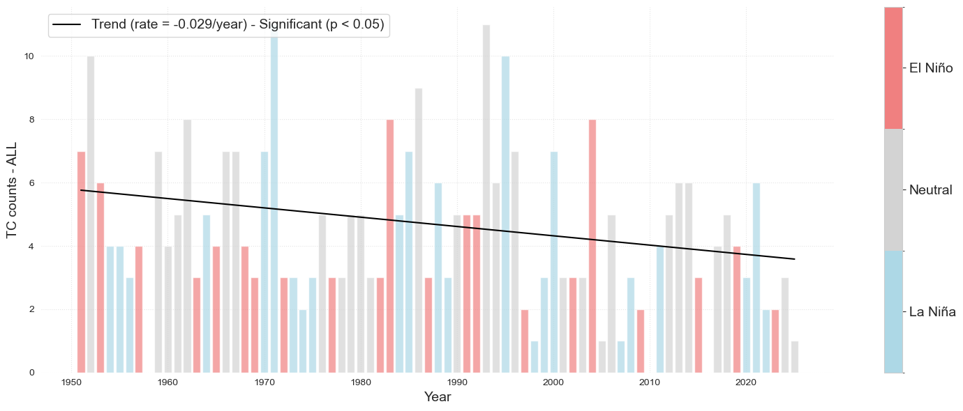
The following bar plot represents the TC counts over time. The color of the bar represents wether it is a El Niño or La Niña year.

ax = plot_bar_probs_ONI(oni_y, 'tc_counts', y_label= 'TC counts - ALL');

The following bar plot represents the severe TC counts over time. The color of the bar represents wether it is a El Niño or La Niña year.

ALL TCs

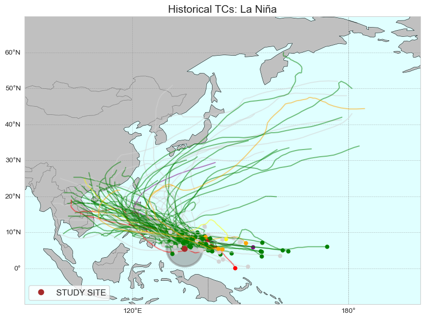
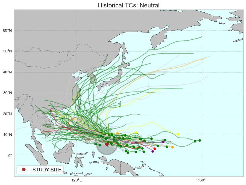
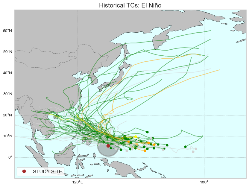
The following plots represent all the TCs in the record for the three different phases of the El Niño Southern Oscillation: “El Niño”, “Neutral” and “La Niña”

names_cat = ['La Niña', 'Neutral', 'El Niño']

for ic, category in enumerate([-1, 0, 1]):

    tcs_cat = tcs_sel.where(tcs_sel_params.oni_cat == category, drop = True)
    tcs_cat_params = tcs_sel_params.where(tcs_sel_params.oni_cat == category, drop = True)

    fig, ax = Plot_TCs_HistoricalTracks_Category(
        tcs_cat, tcs_cat_params.category,
        lon1, lon2, lat1, lat2,
        lon_lat[0], lon_lat[1], r1,
    )
    ax.set_title(f'Historical TCs: {names_cat[ic]}', fontsize=15)

    plt.savefig(op.join(path_figs, f'F9_TCs_{names_cat[ic]}.png'), dpi=300, bbox_inches='tight')

Generate table

Table sumarizing different metrics of the data analyzed in the plots above

from ind_setup.tables import style_matrix, table_tcs_32a, table_tcs_32b

style_matrix(table_tcs_32a(tcs_sel_params, oni), title = 'Key TC Metrics: Vicinity of Palau')

Key TC Metrics: Vicinity of Palau

Metric	Value
Total number of tracks	339.000
Tropical Storms per year	4.644
Standard deviation of storms per year	2.343
Maximum number of storms in a year 1971	11.000
Minimum number of storms in a year 1998	1.000
Major Hurricanes (Category 3+) per year	0.123
Standard deviation of major hurricanes per year	0.331
Maximum number of major hurricanes in a year 1964	2.000
Minimum number of major hurricanes in a year 1959	1.000
EL NIÑO
Total number of storm per year	3.864
Standard deviation of storms per year	1.786
Major Hurricanes (Category 3+) per year	0.000
Standard deviation of severe storms per year
LA NIÑA
Total number of storm per year	4.120
Standard deviation of storms per year	2.552
Major Hurricanes (Category 3+) per year	0.160
Standard deviation of severe storms per year	0.471
NEUTRAL
Total number of storm per year	5.321
Standard deviation of storms per year	2.361
Major Hurricanes (Category 3+) per year	0.179
Standard deviation of severe storms per year	0.000

style_matrix(table_tcs_32b(tcs_WP, oni), title = 'Key TC Metrics: West Pacific Basin')

Key TC Metrics: West Pacific Basin

Metric	Value
Total number of tracks	2664.000
Tropical Storms per year	34.597
Standard deviation of storms per year	7.797
Maximum number of storms in a year 1950	47.000
Minimum number of storms in a year 1982	9.000
Major Hurricanes (Category 3+) per year	6.039
Standard deviation of major hurricanes per year	2.597
Maximum number of major hurricanes in a year 2015	14.000
Minimum number of major hurricanes in a year 1998	1.000
EL NIÑO
Total number of storm per year	32.864
Standard deviation of storms per year	6.405
Major Hurricanes (Category 3+) per year	8.091
Standard deviation of major hurricanes per year	2.575
LA NIÑA
Total number of storm per year	34.920
Standard deviation of storms per year	7.740
Major Hurricanes (Category 3+) per year	5.040
Standard deviation of major hurricanes per year	2.341
NEUTRAL
Total number of storm per year	36.464
Standard deviation of storms per year	7.655
Major Hurricanes (Category 3+) per year	5.750
Standard deviation of major hurricanes per year	1.953